A Pivot Table is an extremely powerful feature in Excel, one that is probably underutilized in many companies. It’s just so cool to be able to move ’tiles’ around and analyze your data a jillion different ways. Even though pivot tables can be sort of intimidating, they’re not hard, and today I’m going to walk you through how to take an unassuming FRx or Management Reporter report and turn it into a powerful pivot table.
Unlike most posts, I’m not going to take you through every single step. Instead, I’m going to hit the main things I’ve learned that will shortcut your experience and hopefully shortcircuit frustration.
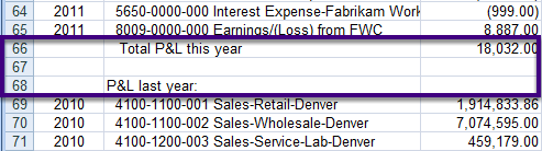
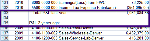
So here’s the unassuming FRx or Management Reporter report:
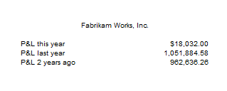
These are year to date numbers for the P&L only for this year, last year, and 2 years ago. You can drill down on these numbers.
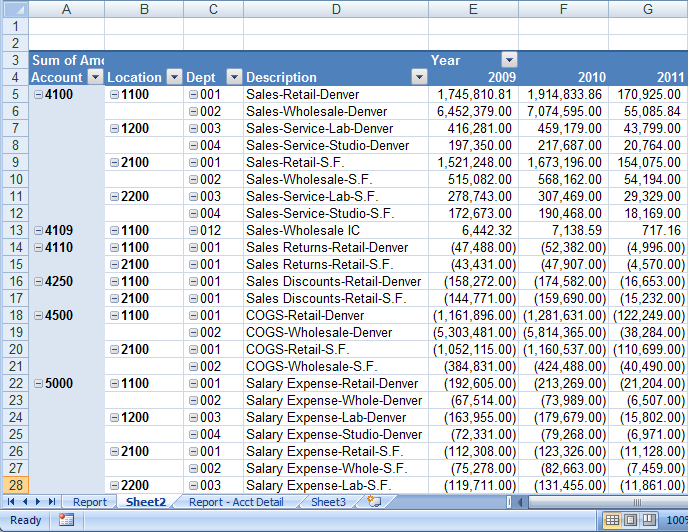
Believe it or not, I’ll turn the FRx or MR summary report into a pivot that looks like this:
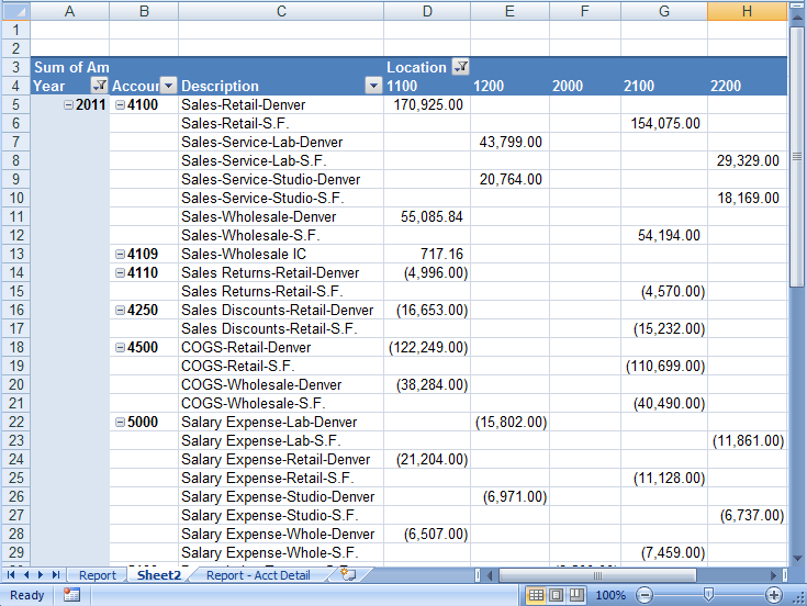
And the same pivot table can also look like this, as well as have many other views:
So next I’ll show you how to get these views and how to set up the FRx or MR report.
The row format in FRx:
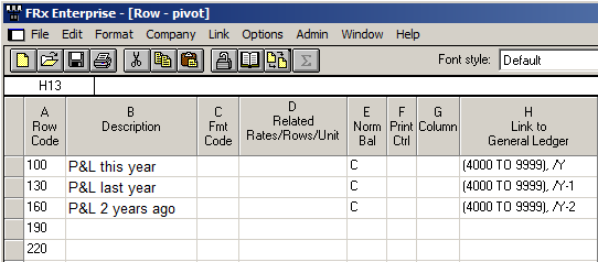
In this example I’m using FRx, but the concepts are exactly the same with Management Reporter. In FRx, you’ll see a range of all P&L accounts, a row modifier /Y, and a sign flip in column E. Same thing with MR, only there’s a separate column in MR for the row modifier that allows you to specify this year, last year, etc.
The column layout in FRx:
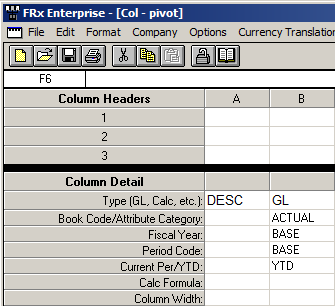
Doesn’t get much simpler than this. In Management Reporter, the Type will be FD (for Financial Data) instead of GL.
The catalog in FRx:
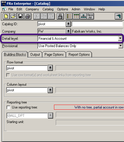
The main thing in the report catalog is to change the Detail level to Financial & Account. If you don’t do this, you won’t have any detail behind those summary numbers.
Export to Excel and the detail raw data will look like this:
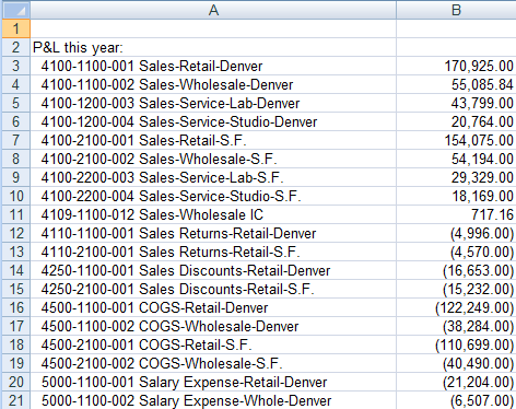
When you export, be sure to select the Account detail option if you’re exporting from the Viewer. Now the edits start.
Edit the data to add headings and the year:
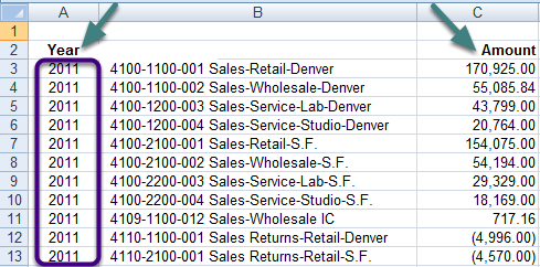
Here I’ll add a couple of column titles, but my primary change is to add the appropriate year to each row through the end of the data.
There are a few rows that need to be deleted:
Delete these rows and the one at the very bottom that totals 2009.
You want to end up with columns of data without any blank or extraneous rows (like headings and totals).
Oh yeah—the F4 key is one of my Excel favorites: it repeats the last edit.
Take a look at the account number and description in column B. There are 4 components in column B, and I’m going to separate each one into its own column:
The account number in my database is composed of Account, Location, and Department. I want to put each of these in its own column. Same for the account description. Here’s how:
- The first step is to insert 3 blank columns to the right of the account-description. The number of columns to insert will depend on the account structure. In this case, I need a total of 4 columns (account, location, department, description), and I already have one (column B), so I’ll add 3 more.
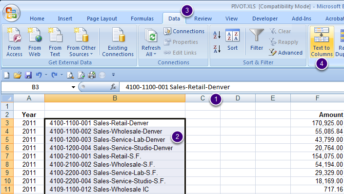
- The next step is to highlight the data in column B. This is the data that you’re going to separate.
- Select the Data tab.
- Choose Text to Columns. This is functionality that lets you separate one Excel cell into separate columns.
The Text to Columns wizard defaults to Delimited, but be sure to choose Fixed width:
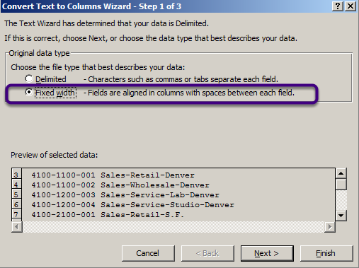
The Fixed Width option will allow you to manually choose where the column breaks should go. In this case, it’s way easier than Delimited.
Use your mouse to click to create column breaks:
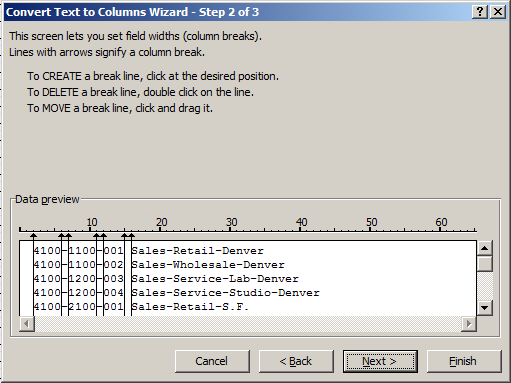
In this example, I’ve used my mouse to click to create 7 lines, giving a total of 8 columns. (I’m not going to ‘import’ all of them though.)
The next step in the wizard allows you to skip columns and to set the type:
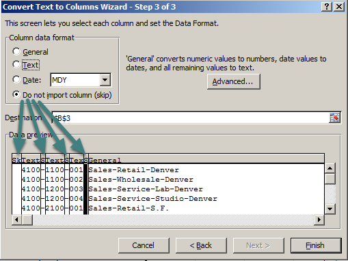
These are the 4 columns that I set to Do not import column (skip). They contain the extra spaces preceding the account number, the hyphens separating the account numbers, and the extra spaces preceding the description. So they are definitely not needed.
By the same token, there are 3 account number columns, and I set them to Text. They default to General. If you change these to Text, you will thank me later when they magically drop into the pivot table in exactly the right place.
I let the description column default to General because Excel will already know that it’s text, and it saves me a click or two.
(An aside to Excel gurus—sometimes I parse this using the Excel functions left, mid, and right, but Text to Columns is easier to understand and less prone to errors for those who’ve never done this before.)
The data after Text to Columns. Cool, huh.
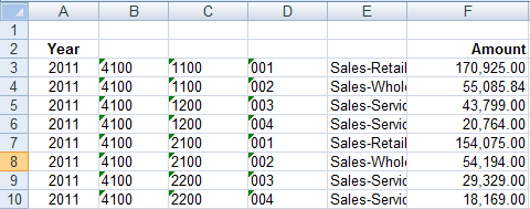
I love Text to Columns.
Add column descriptions:
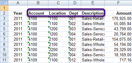
I’ve added the column headings as needed for the 4 new columns.
I like to Format as Table before moving on to create the pivot:
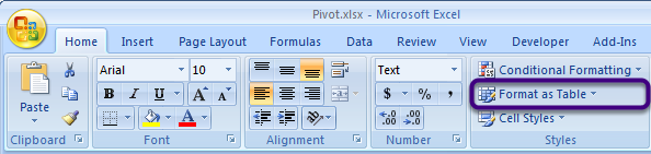
Click anywhere inside the data, then Format as Table.
Excel automatically chooses the data for you.
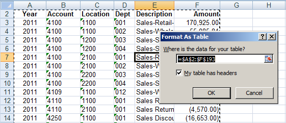
Be sure to check My table has headers. It might be a good idea to check to see that all your data is included, because if there are any blank rows, you need to get rid of them before continuing.
Under Table Tools, Design, Quick Styles, I have None selected. That’s why the rows don’t have alternating shading like tables usually do.
The data formatted as a table. Ready for the pivot!
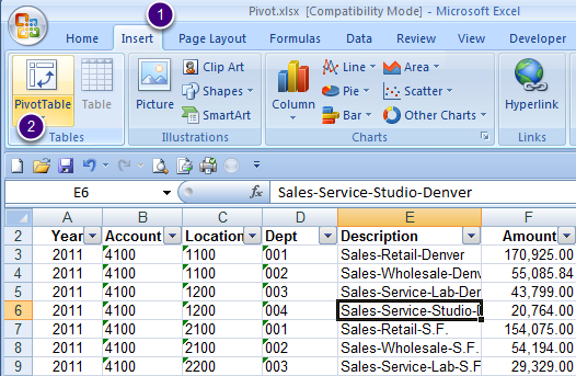
Click anywhere inside the table:
- Select the Insert tab
- Choose PivotTable
I usually let this default and just click OK:
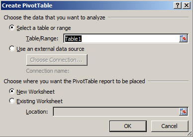
Your range is already selected, because by default Excel uses the table you just created.
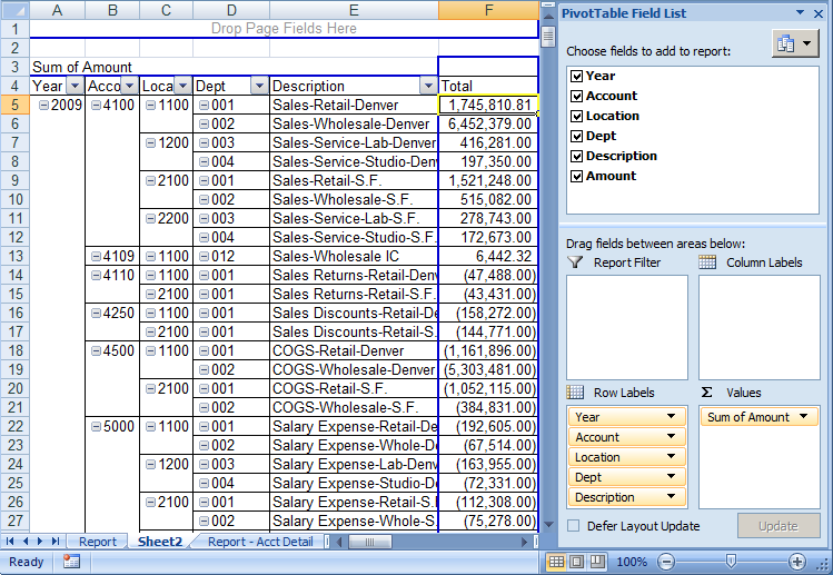
This is where most people get intimidated:
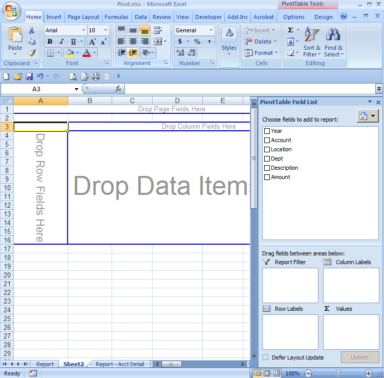
For the time being, I’m just going to click all 6 Fields and just see where they land:
Watch where the ‘Tiles’ appear at the bottom when you check each field box.
Remember when I did Text to Columns and marked those account numbers as text? Well this is where that pays off. Excel sees them as text and puts them under Row Labels.
Tip: Most people find it far easier to move Tiles in the bottom right hand corner than dropping data fields onto the pivot table itself.
Notice Excel also sees my Year column, thinks it’s a number, and automatically sums its value. That will be my first change.
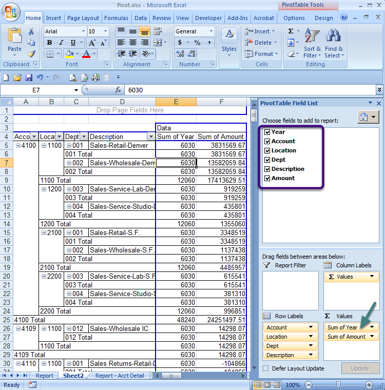
In this screenshot, I’ve dragged Sum of Year over to top of the Row Labels:
So now I’ve got a great start to a pivot table. But there are a couple things that drive me crazy about this, not the least of which is the Total column without any commas. I also don’t like all the subtotals—too messy.
First I’ll turn off subtotals:
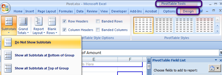
Take a look at PivotTable Tools—on the Design tab, there is a Subtotals icon. I’ll choose the option Do Not Show Subtotals. I also turned off Grand Totals on the icon next door.
Then I’ll turn on commas:
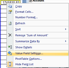
Click one of the numbers in the Total column, right click and choose Value Field Settings.
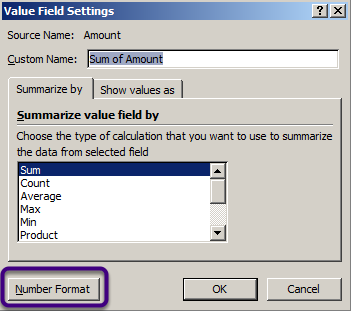
Click the Number Format button.
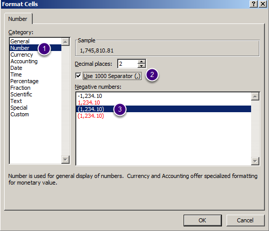
I made 3 changes here. I changed from General to Number, checked the box for Use 1000 Separator, and I changed the format for negative numbers.
This is starting to shape up:
What a relief—the amounts have commas and 2 decimal places.
Note that my example is far more “scrunched up” than normal due to blog space considerations.
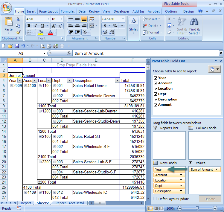
Finishing touches—apply a style, and make the first pivot:
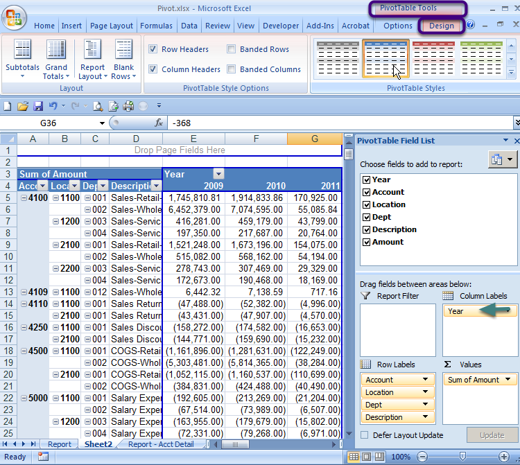
On the PivotTable Tools menu, on the Design tab, in the PivotTable Styles section, you can choose any Style you want. I chose Pivot Style Medium 9 for this one.
Then I grabbed the Year tile from the Row Label section, and moved it over to the Column Label section. And the result is the pivot that I showed at the top of this post.
But the possibilities are mind boggling!
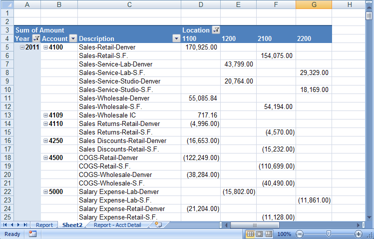
Here’s one more pivot:
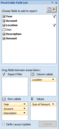
I’ve filtered the year—I only want to see 2011.
I’ve filtered the location—I turned off a couple of locations without data.
I’ve unchecked department—don’t want to see it at all.
I’ve moved the year back to the Rows.
I’ve moved the Location to the Columns.
Voila!
That’s enough for one day, but I hope you can see the amazing possibilities of how you can drag and drop and look at your data in so many different ways. All from a very simple-looking FRx or Management Reporter summary report with drilldown to account detail enabled.
One other thing—those in IT might wonder why I don’t go straight to the ERP from Excel. I started with FRx (or Management Reporter) because it is already linked to the ERP and all I had to do was just pull the full range of P&L accounts using a very simple report. I don’t have to worry about configuring ODBC, what tables to use, what fields to pull, how to link the tables, right joins, left joins, inner joins, and so on.
Enjoy your pivots. Cheers—Jan
Hello Jan,
Discovering this article made my day! I have been asking our IT dept. to update excel in order to use pivot tables they way you taught in this article.
Happy Holidays,
William
Thrilled to hear it!